How to Find the Cell Reference for a Searched Value in an Array in Excel

John Ormsby (aka NASANUT) sent in what he playfully called a Dumb Question:

I have a spreadsheet that contains a 10 by 10 matrix of values. Each value is different. There are column headings at the top, ranging from 0 to 9 and there are row headings on the left, also ranging from 0 to 9.

What I want to do is this. I want to search for a value within the matrix, and if found, want Excel to tell me the row and column that it is in. In other words, if I search the matrix for ‘150’ and it is found at cell F7, then Excel can either tell me ‘F7’ or the row and column headings (I can work with either).

The problem I have is that all of my searching only results in information on how to go the other way (i.e. provide the column and row and ‘find’ the value).

The beautiful thing about this question is that a) it’s not at all dumb, it’s a surprisingly hard problem, and b) I had a lot of other things on my to do list (some of them fairly urgent) but of course I dropped everything to try to figure this out!

When I first went searching for a way to return the cell reference (aka F7), I found a function called ADDRESS. At first blush it appears to be exactly what we want. If we enter the formula:

=ADDRESS(cellRow,cellColumn)

Using 7,6 as the row and column, it will indeed return F7. That’s really swell, but how do we figure out what the row and column numbers are? That’s when things got seriously tricky.

Mike Rickson in the mrexcel.com forum gave me the basic idea of how to attack the problem. I changed a bit of what he did to suit our specific need.

I’m going to step through all of this breaking down each step, but at the end you will only need one elegant but long command to perform this entire function. At the very end of this explanation is an Excel file you can download so you can play with it yourself to see how it works. Ok, ready for some geekery?

Unary Operator

Mike’s solution makes use of something called a double unary operator. Bart taught us about unary operators in JavaScript but it seems to work differently in Excel. In this instance, we’ll be using a minus symbol as a unary operator.

If you have a positive 6 in cell B7 and you create a formula that says
=-B7

it will return -6.

If you have a negative 6 in cell B7, it will return 6. It’s simply switching the sign.

What if you use the negative/hyphen/minus/unary operator twice? With regular numbers, the two cancel each other out, so — applied to 6 gives you back 6, and — applied to -6 returns -6.

So far, that’s pretty obvious. But what happens if you apply the unary operator to TRUE/FALSE values? By some mysterious convention decided on a long time ago, – applied to TRUE coerces the value to -1, and – applied to FALSE coerces it’s value to 0. That’s the actual term, “coerce”.

If you use the negative/hyphen/minus/unary operator twice, it first coerces the TRUE/FALSE to -1/0, and the second – just flips the sign like any other number. So – applied to TRUE coerces to -1, and the second – flips the sign so you get positive 1. Nothing interesting happens to FALSE when you apply the unary operator twice though, since it’s already 0.

At the risk of saying two wrongs made a right, is everyone still with me?

Using the Unary Operator to Make an Array

We’re going to run some functions to search for our value in the array. Normally this would return an array of TRUE/FALSE values. But with our handy unary operator, we can return a new array that has all 0s, except where it finds our value and in that position it will place a 1.

So why does THAT help us at all? We need a second array before it will all become clear. Our next array makes use of the ROW function. We point the ROW function at the original array and it returns an array where every row simply repeats the row number. It will have 1,1,1,1 in the first row, 2,2,2,2, in the second row.

Note that the ROW function returns the absolute row reference, not the row within your range.

Now, armed with our two arrays, one with all 0s except a 1 where the searched value was, and one with the row numbers, we can finally get something done. If we multiply the two arrays against each other, all the 0s will stay 0s, but the 1 will turn into the row number. We now know the row number of our searched value. But it’s still buried in an array.

An array with that one cell showing us the row value isn’t that helpful, we need it all by itself. Instead of multiplying our two matrices together, if we do a SUMPRODUCT of the two matrices, it will drop out a single value, the row number of our found value! If we repeat using COLUMN instead of ROW, we will have both values to plop into our original ADDRESS function to find the cell reference of the found value (which was our original objective).

Let’s walk through an example.

We will name the range of values we’re searching to be called dataRange. If this is our dataRange:

11	22	33
44	55	66
77	88	99

First, select an empty range of cells in your spreadsheet that’s the same size as dataRange (same number of rows and columns). With that new range of cells selected, if we want to find the location of the value 66 enter the following:

--(dataRange=66)

And hit Control-Shift-Enter. When you hit CSE (as it’s referred to by all the cool kids), the formula will now have braces around it, showing that it’s an “array function”.

{--(dataRange=66)}

You now should see the following in your new array::

0	0	0
0	0	1
0	0	0

Select another empty region the same size as our original and enter this formula (followed by CSE):

={ROW(dataRange)}

And assuming our original array is in the top left corner, it will return the array:

1	1	1
2	2	2
3	3	3

Now if we multiply these two arrays together, again selecting a new range of cells the same size as our original:

={--(dataRange=66)*ROW(dataRange)}

we would get the array:

0	0	0
0	0	2
0	0	0

Instead, let’s do the SUMPRODUCT of the two arrays (which does not create a new array and so does not require selection of an empty region nor does it require CSE.

={SUMPRODUCT(--(dataRange=66)*ROW(dataRange))}

returns the value of 2.

We now know that 66 is in row 2 of our range.

Running this again only with COLUMN gives us column 3 for our found value:

={SUMPRODUCT(--(dataRange=66)*COLUMN(dataRange))

returns the value of 3 is the column number.

Now with our amazing knowledge that 66 is in row 2, column 3, we can finally convert that into the cell reference designation by entering those two values into the ADDRESS function.

=ADDRESS(2,3)

returns $C$2.

Note that the dollar symbol in front both the column and row designations means this is the absolute location. However, if you select your dataRange and move it to another location in the sheet, the cell reference designation returned by the formula will still update to the new information.

We can combine all of these formula bits and pieces together into one giant formula of doom (™Donald Burr). Note that I’ve created another variable called myValue which is the value for which we’re searching.

The One, Long, Elegant Formula!

=ADDRESS(SUMPRODUCT(--(datarange=myValue)*ROW(datarange)),SUMPRODUCT(--(datarange=myValue)*COLUMN(datarange)))

I want to add one caveat to this entire exercise, this works only if the values in the array are unique. Otherwise, it barfs out a nonsense location not even IN the array! I’m betting someone clever will make a comment below explaining how to have it error out in a more sensible way.

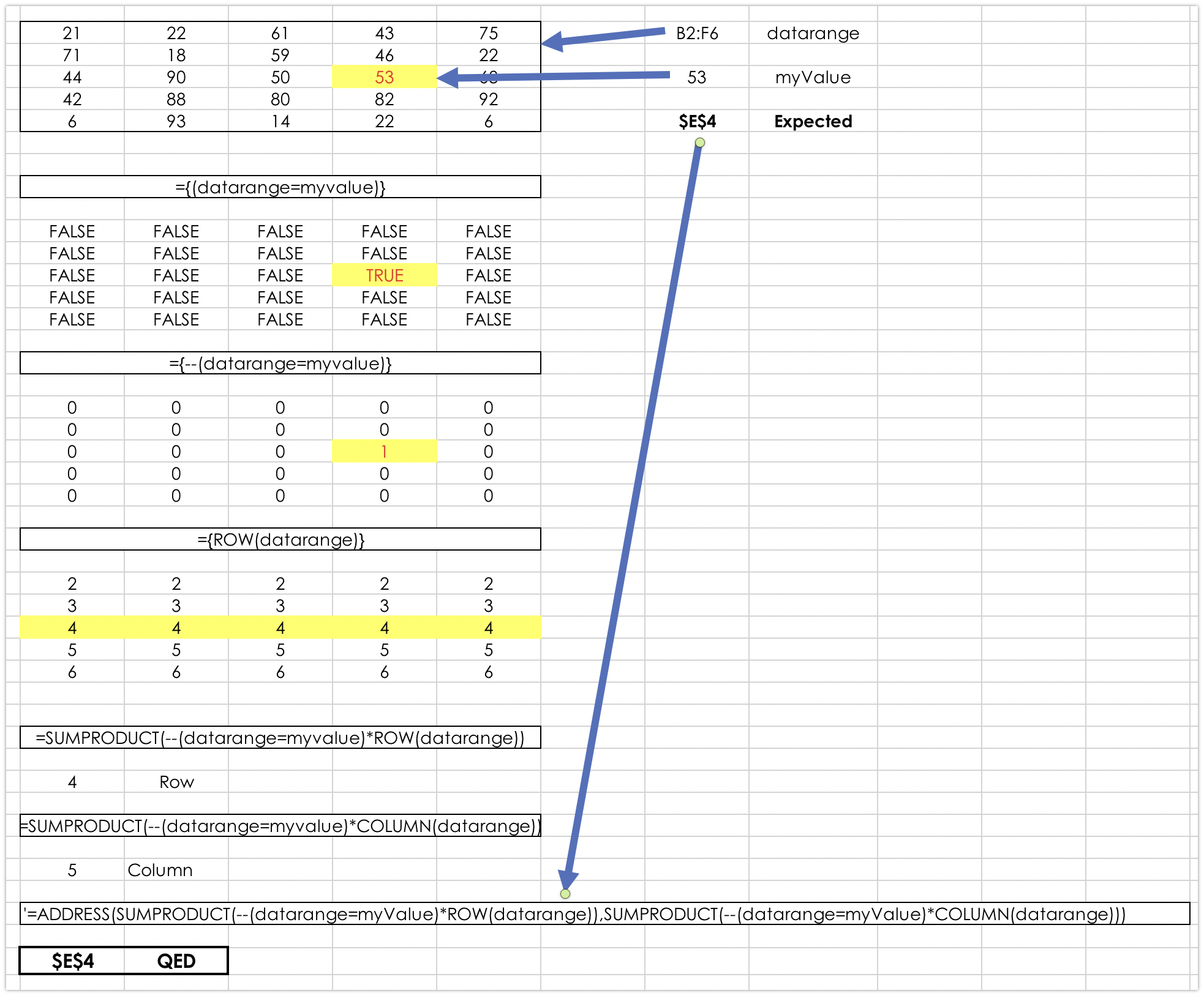
If you’d like to download an example spreadsheet where I break it down step by step. You can download it from my OneDrive account here: 1drv.ms/…

Here’s a screenshot of the downloadable spreadsheet: